Kalman Filter Explained with MATLAB Code

The Kalman Filter is a recursive algorithm for estimating the state of a dynamic system from noisy observations. Developed by Rudolf E. Kálmán in 1960, it's widely used in robotics, navigation, aerospace, finance, and more.

What is the Kalman Filter?

The Kalman Filter maintains a probabilistic (Gaussian) estimate of the system state over time, updating recursively with each new measurement using two steps:

Prediction Step

x̂_k|k-1 = F_k * x̂_k-1|k-1 + B_k * u_k
P_k|k-1 = F_k * P_k-1|k-1 * F_k^T + Q_k

Update Step

K = P_k|k-1 * C^T * (C * P_k|k-1 * C^T + R)^-1
x̂_k = x̂_k|k-1 + K * (y_k - C * x̂_k|k-1)
P_k = (I - K * C) * P_k|k-1

MATLAB Code: Estimating Position with Constant Acceleration

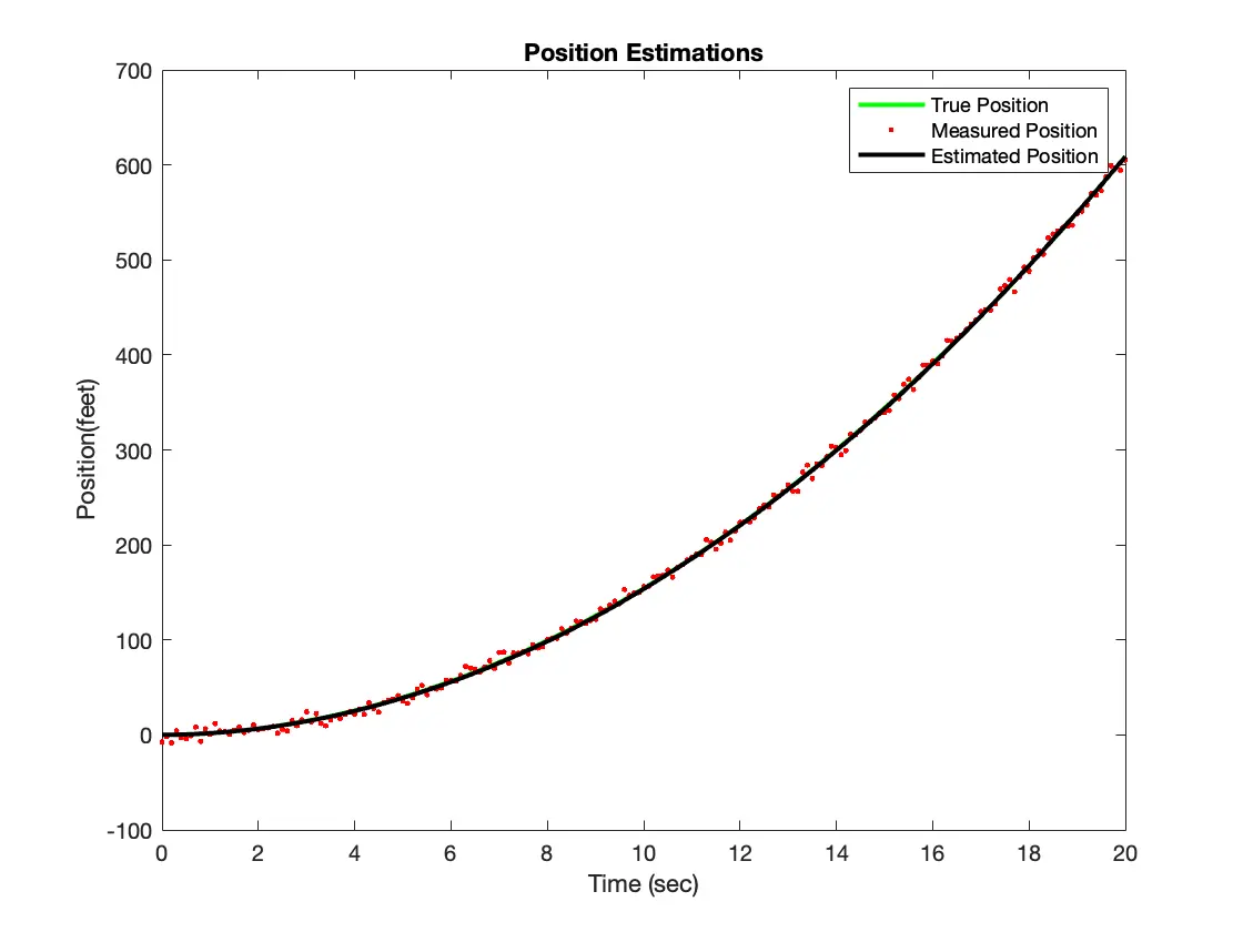
Problem: A vehicle has an acceleration of 3 ft/sec², position measured every 0.1 seconds with 5 ft noise, acceleration noise of 0.1 ft/sec². Estimate position over 20 seconds.

clc; clear;

duration = 20;
dt = 0.1;
measnoise = 5;       % position measurement noise (feet)
accelnoise = 0.1;    % acceleration noise (feet/sec^2)

A = [1 dt; 0 1];     % transition matrix
B = [dt^2/2; dt];    % input matrix
C = [1 0];           % measurement matrix
x = [0; 0];          % initial state
xhat = x;            % initial estimate

Sz = measnoise^2;
Sw = accelnoise^2 * [dt^4/4 dt^3/2; dt^3/2 dt^2];
P = Sw;

tpos = []; poshat = []; posmeasured = [];

for t = 0:dt:duration
    u = 3; % constant acceleration
    ProcessNoise = accelnoise * [(dt^2/2)*randn; dt*randn];
    x = A*x + B*u + ProcessNoise;

    MeasNoise = measnoise * randn;
    y = C*x + MeasNoise;

    xhat = A*xhat + B*u;
    Inn = y - C*xhat;
    s = C*P*C' + Sz;
    K = A*P*C' * inv(s);
    xhat = xhat + K*Inn;
    P = A*P*A' - A*P*C'*inv(s)*C*P*A' + Sw;

    tpos = [tpos; x(1)];
    posmeasured = [posmeasured; y];
    poshat = [poshat; xhat(1)];
end

t = 0:dt:duration;
figure;
plot(t, tpos, 'g', 'LineWidth', 2); hold on;
plot(t, posmeasured, 'r.', 'LineWidth', 2);
plot(t, poshat, 'k', 'LineWidth', 2);
title('Position Estimations');
xlabel('Time (sec)'); ylabel('Position (feet)');
legend('True Position', 'Measured Position', 'Estimated Position');

Applications

Navigation & GPS systems
Robotics and autonomous vehicles
Aerospace and flight control
Financial time series estimation
Signal processing and sensor fusion

References

R. E. Kalman, "A new approach to linear filtering and prediction problems," ASME Journal of Basic Engineering, 1960.
G. Welch & G. Bishop, "An introduction to the Kalman filter," UNC Chapel Hill, 2006.